Нейромодель RF-PSTH (симулирующая структуру рецептивного поля (РП) и выходной нейронный сигнал PSTH)

English Русский Français

Бесплатный учебный инструмент для студентов, преподавателей и ученых, работающих в областях нейробиологии, биоинформатики, биофизики, биомедицинской инженерии и искусственного интеллекта.

Краткое содержание

Существующие на сегодняшний день модели искусственных нейронов не способны моделировать фундаментально важные свойства биологических нейронов:
1) антагонистические рецептивные поля и
2) выходной ответный сигнал нейрона PSTH на любой стимул (раздражитель).
Даже если некоторые модели нейронов и пытаются моделировать антагонистические рецептивные поля, то они не способны моделировать выходной сигнал PSTH, и наоборот – при попытке определенных моделей моделировать выходной сигнал нейрона PSTH, они не в состоянии разъяснить происхождение антагонистических рецептивных полей нейронов.
Например, одна из самых популярных моделей DOG (Difference Of Gaussians) моделирует антагонистическую структуру рецептивного поля, однако не способна моделировать выходной сигнал нейрона PSTH.
Подавляющее большинство моделей искусственных нейронов не способны моделировать ни антагонистические рецептивные поля нейронов, ни выходные сигналы PSTH нейрона.
Впервые в истории нейробиологии модель нейрона RF-PSTH способна моделировать как антагонистические рецептивные поля нейронов, так и выходной сигнал PSTH.
Нейромодель RF-PSTH основана на физических свойствах биологических нейронов.


Рекомендуемая литература

Подробное описание рецептивного поля биологического нейрона изложено в книге «Encyclopedia of the Human Brain», автор книги: Вилейанур Рамачандран (англ. Vilayanur S. Ramachandran) (редактор), издательство: «Academic Press», 10 июля 2002 г. (1-ое издание), ISBN-10: 0122272102, ISBN-13: 978-0122272103.
В этой книге, пожалуйста, прочитайте главу «Receptive Field», написанную Rajesh P. N. Rao (University of Washington), страницы 155-168.
Нейромодель RF-PSTH симулирует функции нейрона, описанные в этой главе.

Значение и преимущества новой нейромодели RF-PSTH

Генерируемый нейромоделью RF-PSTH выходной сигнал PSTH соответствует данным экспериментальных, лабораторных измерений реальных биологических нейронов.
Измерения реальных биологических нейронов показывают, что рецептивные поля сенсорных нейронов имеют симметричную, антагонистическую структуру концентрических кругов, однако современная наука не может удовлетворительно объяснить причину этого феномена. Высказываются гипотеза, что антагонистические, концентрические рецептивные поля формируются из-за того, что нейрон соединяется с рецепторами (или другими нейронами) посредством синаптических соединений, и предположительно эти синаптические соединения распределяются таким образом, что формируются антагонистические концентрические круги. Не существует удовлетворительного объяснения того, почему рецептивные поля должны формировать антагонистические структуры в форме концентрических кругов.
Нейромодель RF-PSTH может симулировать антагонистические, концентрические круговые структуры рецептивных полей сенсорных нейронов.
Нейромодель RF-PSTH утверждает, что антагонистическая круговая структура рецептивного поля является внутренней особенностью всех сенсорных нейронов, и для формирования такой структуры не требуется никаких внешних нейронных связей (внешних нейронных сетей).


Программа нейромодели RF-PSTH


По ниже приведенным ссылкам можно скачать программу «Нейромодель RF-PSTH» v.2.5 для следующих платформ:

Пробную версию Нейромодели RF-PSTH можно свободно использовать в академических и образовательных целях.


Описание Нейромодели RF-PSTH

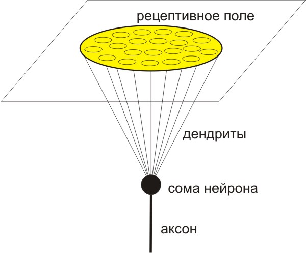
Нейрон имеет тело (сому), дендриты и аксоны.

Нейрон моделируется как трехмерный объект в трехмерном пространстве:
1) сома нейрона моделируется как математическая точка;
2) рецептивное поле нейрона моделируется как двумерная плоскость;
3) дендриты, исходящие из сомы нейрона, достигают двумерной плоскости;
4) в двумерной плоскости дендриты формируют круговое рецептивное поле;
5) трехмерная форма нейрона является прямым круговым конусом, вершина которого репрезентирует сому нейрона, а основание – рецептивное поле.

Такой вариант хорошо иллюстрируется на примере ганглиозной (нейронной) клетки, получающей входные сигналы от фоторецепторов в сетчатке. Большинство других нейронов также довольно неплохо соответствуют этой модели, например, соматосенсорные нейроны, получающие входные сигналы от кожи, и т.д.

Пошаговые инструкции по запуску программы нейромодели RF-PSTH

Этап #1

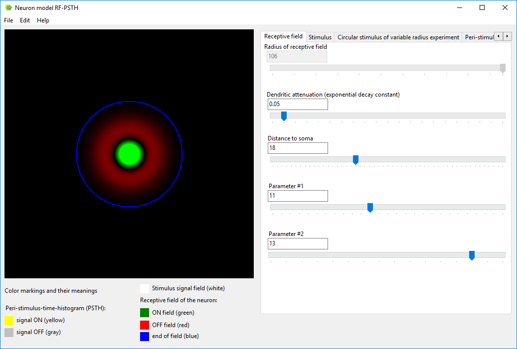
Выберите параметры, определяющие структуру рецептивного поля нейрона. Их можно выбрать во вкладке под названием «Рецептивное поле» (“Receptive field”).
Параметры нейрона являются такими:
Радиус рецептивного поля (Radius of receptive field) – этот параметр рассчитывается автоматически, вам не надо выбирать его значение;
Затухание дендритов (константа экспоненциального убывания) (Dendritic attenuation (exponential decay constant)) – когда сигнал распространяется по дендритам, он затухает по закону экспоненциального убывания, при помощи этого параметра устанавливается константа экспоненциального убывания;
Расстояние до сомы (Distance to soma) – расстояние от сомы до плоскости рецептивного поля;
Параметр #1 (Parameter #1) – параметр, устанавливающий диаметр дендритов;
Параметр #2 (Parameter #2) – еще один параметр нейрона.



Рисунок 2. Вкладка «Рецептивное поле» (“Receptive field”) в программе нейромодели RF-PSTH.

Этап #2

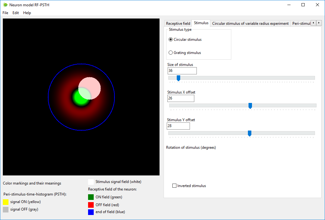
Создайте стимул с нужными параметрами. Это можно осуществить во вкладке под названием «Стимул» (“Stimulus”).
Стимул изображается белым цветом на рецептивном поле нейрона.

Стимул может быть нескольких типов:
1) круговой стимул (circular stimulus) – вы можете выбрать радиус и координаты центра круга (x,y);
2) стимул-решетка (grating stimulus) – вы можете выбрать ширину решетки, координаты параллельного переноса (x,y) и угол поворота (в градусах);
3) инвертированный стимул (inverted stimulus) – инверсия стимулированных и не стимулированных областей.

Параметры кругового стимулы можно менять непосредственно мышкой (менять размер и перемещать), нажав кнопкой мышки на образ стимула.
Стимул-решетку можно изменять только при помощи скользящей метки (sliding trackbar) в нижеприведенных диапазонах значений.
С помощью нейромодели RF-PSTH также можно симулировать реакцию нейрона на движущийся стимул, однако в этой версии программы можно симулировать только статические, не движущиеся стимулы.


Рисунок 3. Вкладка «Стимул» (“Stimulus”) в программе нейромодели RF-PSTH.

Этап #3

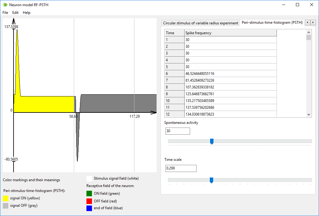
Симулируйте выходной сигнал нейрона как реакцию на входной стимул. Это можно выполнить во вкладке под названием «Временная перистимульная гистограмма» (“Peri-stimulus-time-histogram (PSTH)”).
Стимул включается, когда время равно нулю. Стимул выключается автоматически, когда выходной сигнал нейрона стабилизируется и становится почти стационарным. Выходной сигнал нейрона отображается желтым цветом, когда стимул включен, и серым при выключенном стимуле.


Рисунок 4. Вкладка «Временная перистимульная гистограмма» (“Peri-stimulus-time-histogram (PSTH)”) в программе нейромодели RF-PSTH.

Дополнительные замечания о выходном сигнале PSTH

Реальные биологические нейроны не могут генерировать потенциалов действия с отрицательной частотой в своих выходных сигналах. Однако этот отрицательный выходной сигнал можно измерять как уменьшенный пресинаптический потенциал внутри сомы нейрона, находящийся в месте, где аксон соединяется с сомой. Данная симуляционная программа показывает и раскрывает происходящие в нейроне внутренние процессы.

Выходной сигнал PSTH рассчитывается без учета кратковременной депрессии (STD) и кратковременной фасилитации (содействия) (STF).

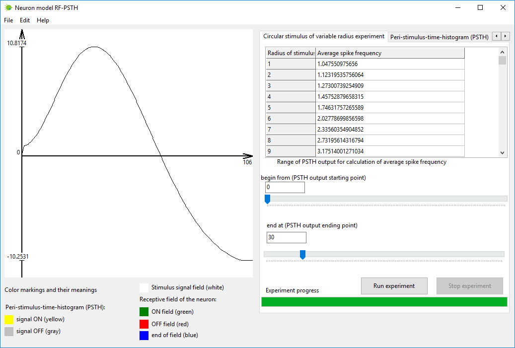
Этап #4

Симулируйте эксперимент с круговым стимулом переменного радиуса. Это можно выполнить во вкладке «Эксперимент с круговым стимулом переменного радиуса» (“Circular stimulus of variable radius experiment”).

Описание эксперимента является следующим. Круговой стимул помещается в центр рецептивного поля. Размер стимула увеличивается пошагово, начиная с нуля и заканчивая размером рецептивного поля. На каждом шаге вычисляется выходной сигнал PSTH. На каждом шаге берется диапазон выходных значений из графика PSTH и вычисляется средняя частота потенциалов действия для этого определенного диапазона. Конечный график, получающийся в результате эксперимента, изображает зависимость средней частоты потенциалов действия от размера стимула. Форма конечного графика чувствительна к выбранному диапазону выходного сигнала PSTH, на основе которого вычисляется средняя частота потенциалов действия. Изменение выбранного диапазона (выходного сигнала PSTH) меняет конечный график эксперимента. В нейронауке не существует правил, которые определяли бы, какой диапазон сигнала PSTH следует выбрать для вычисления средней частоты потенциалов действия. Поэтому вам следует самим поэкспериментировать со значениями этого диапазона для того, чтобы найти такой диапазон, который лучше всего соответствовал бы вашим целям.


Рисунок 5. Вкладка «Эксперимент с круговым стимулом переменного радиуса» (“Circular stimulus of variable radius experiment”) в программе нейромодели RF-PSTH.


Недостатки современных моделей искусственных нейронов и превосходство нейромодели RF-PSTH

Математическое моделирование любого физического феномена требует упрощений (редукций) этого феномена для того, чтобы уменьшить количество моделируемых параметров и количество вычислений. Технический вопрос состоит в том, насколько данный феномен можно упростить, чтобы не потерять важную информацию, нужную для решения конкретной задачи.
Например, если нам нужно проанализировать движение автомобиля по дороге, мы можем редуцировать автомобиль до математической точки (не имеющей размеров и массы), которая движется через двумерное пространство с некоторой скоростью. Такая упрощенная модель автомобиля годится для того, если мы хотим, к примеру, рассчитать, сколько времени у автомобиля уйдет на переезд из точки А в точку Б. Однако, если нам надо выяснить, какая сила воздействует на тормозные диски автомобиля, когда водитель нажимает на тормозные педали для остановки машины, то тогда модели, в которой автомобиль отображается как математическая точка, будет недостаточно для решения такой задачи. Если вам требуется выяснить, какая сила действует на тормозные диски автомобиля, когда водитель нажимает на тормозную педаль, то тогда вам надо знать массу автомобиля, диаметр колес, и т.д. – но все эти параметры были исключены из описанной выше модели автомобиля. Другими словами, при создании математической модели можно исключить некоторые существенные особенности (параметры), без которых будет невозможно решить некоторые специфические практические задачи.

Рассмотрим более подробно используемые на сегодняшний день модели искусственных нейронов.

http://en.wikipedia.org/wiki/Artificial_neuron

History The first artificial neuron was the Threshold Logic Unit (TLU) first proposed by Warren McCulloch and Walter Pitts in 1943. As a transfer function, it employed a threshold, equivalent to using the Heaviside step function. Initially, only a simple model was considered, with binary inputs and outputs, some restrictions on the possible weights, and a more flexible threshold value. Since the beginning it was already noticed that any boolean function could be implemented by networks of such devices, what is easily seen from the fact that one can implement the AND and OR functions, and use them in the disjunctive or the conjunctive normal form. Researchers also soon realized that cyclic networks, with feedbacks through neurons, could define dynamical systems with memory, but most of the research concentrated (and still does) on strictly feed-forward networks because of the smaller difficulty they present. One important and pioneering artificial neural network that used the linear threshold function was the perceptron, developed by Frank Rosenblatt. This model already considered more flexible weight values in the neurons, and was used in machines with adaptive capabilities. The representation of the threshold values as a bias term was introduced by Bernard Widrow in 1960. In the late 1980s, when research on neural networks regained strength, neurons with more continuous shapes started to be considered. The possibility of differentiating the activation function allows the direct use of the gradient descent and other optimization algorithms for the adjustment of the weights. Neural networks also started to be used as a general function approximation model. 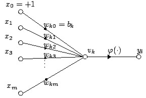<...> Basic structure For a given artificial neuron, let there be m + 1 inputs with signals x0 through xm and weights w0 through wm. Usually, the x0 input is assigned the value +1, which makes it a bias input with wk0 = bk. This leaves only m actual inputs to the neuron: from x1 to xm. 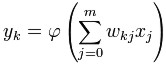The output of kth neuron is: Where φ is the transfer function. The output is analogous to the axon of a biological neuron, and its value propagates to input of the next layer, through a synapse. It may also exit the system, possibly as part of an output vector. It has no learning process as such. Its transfer function weights are calculated and threshold value are predetermined. <...> Types of transfer functions The transfer function of a neuron is chosen to have a number of properties which either enhance or simplify the network containing the neuron. Crucially, for instance, any multilayer perceptron using a linear transfer function has an equivalent single-layer network; a non-linear function is therefore necessary to gain the advantages of a multi-layer network. 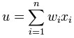Below, u refers in all cases to the weighted sum of all the inputs to the neuron, i.e. for n inputs, where w is a vector of synaptic weights and x is a vector of inputs. 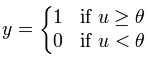Step function The output y of this transfer function is binary, depending on whether the input meets a specified threshold, θ. The "signal" is sent, i.e. the output is set to one, if the activation meets the threshold. This function is used in perceptrons and often shows up in many other models. It performs a division of the space of inputs by a hyperplane. It is specially useful in the last layer of a network intended to perform binary classification of the inputs. It can be approximated from other sigmoidal functions by assigning large values to the weights. Linear combination In this case, the output unit is simply the weighted sum of its inputs plus a bias term. A number of such linear neurons perform a linear transformation of the input vector. This is usually more useful in the first layers of a network. A number of analysis tools exist based on linear models, such as harmonic analysis, and they can all be used in neural networks with this linear neuron. The bias term allows us to make affine transformations to the data. Sigmoid A fairly simple non-linear function, a Sigmoid function such as the logistic function also has an easily calculated derivative, which can be important when calculating the weight updates in the network. It thus makes the network more easily manipulable mathematically, and was attractive to early computer scientists who needed to minimize the computational load of their simulations. It is commonly seen in multilayer perceptrons using a backpropagation algorithm. <...> Comparison to biological neurons Artificial neurons bear a striking similarity to their biological counterparts. Dendrites - In a biological neuron, the dendrites act as the input vector. These dendrites allow the cell to receive signals from a large (>1000) number of neighboring neurons. As in the above mathematical treatment, each dendrite is able to perform "multiplication" by that dendrite's "weight value." The multiplication is accomplished by increasing or decreasing the ratio of synaptic neurotransmitters to signal chemicals introduced into the dendrite in response to the synaptic neurotransmitter. A negative multiplication effect can be achieved by transmitting signal inhibitors (i.e. oppositely charged ions) along the dendrite in response to the reception of synaptic neurotransmitters. Soma - In a biological neuron, the soma acts as the summation function, seen in the above mathematical description. As positive and negative signals (exciting and inhibiting, respectively) arrive in the soma from the dendrites, the positive and negative ions are effectively added in summation, by simple virtue of being mixed together in the solution inside the cell's body. Axon - The axon gets its signal from the summation behavior which occurs inside the soma. The opening to the axon essentially samples the electrical potential of the solution inside the soma. Once the soma reaches a certain potential, the axon will transmit an all-in signal pulse down its length. In this regard, the axon behaves as the ability for us to connect our artificial neuron to other artificial neurons. Unlike most artificial neurons, however, biological neurons fire in discrete pulses. Each time the electrical potential inside the soma reaches a certain threshold, a pulse is transmitted down the axon. This pulsing can be translated into continuous values. The rate (activations per second, etc.) at which an axon fires converts directly into the rate at which neighboring cells get signal ions introduced into them. The faster a biological neuron fires, the faster nearby neurons accumulate electrical potential (or lose electrical potential, depending on the "weighting" of the dendrite that connects to the neuron that fired). It is this conversion that allows computer scientists and mathematicians to simulate biological neural networks using artificial neurons which can output distinct values (often from -1 to 1).

Wikipedia

Все эти модели искусственных нейронов не могут объяснить и симулировать антагонистические рецептивные поля и выходной сигнал PSTH реальных биологических нейронов. На основе таких недействительных искусственных нейронов строятся Искусственные Нейронные Сети.
Если Искусственная Нейронная Сеть (ИНС) строится из нейронов с линейной передаточной функцией, то тогда такую многослойную сеть можно упростить до однослойной сети, которая будет эквивалентна исходной многослойной сети. Поэтому нелинейная передаточная функция создает преимущества для многослойной сети.

http://www.cs.bham.ac.uk/~jxb/INC/l7.pdf

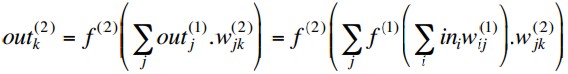
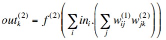
The Need For Non-Linearity We have noted before that if we have a regression problem with non-binary network outputs, then it is appropriate to have a linear output activation function. So why not simply use linear activation functions on the hidden layers as well? With activation functions f(n)(x) at layer n, the outputs of a two-layer MLP are so if the hidden layer activations are linear, i.e. 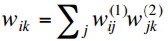f(1)(x) = x, this simplifies to But this is equivalent to a single layer network with weights and we know that such a network cannot deal with non-linearly separable problems.

Learning in Multi-Layer Perceptrons - Back-Propagation Neural Computation : Lecture 7 John A. Bullinaria, 2013

Если в построении искусственного нейрона будет использоваться линейная передаточная функция, и если количество входных нейронных сигналов будет сведено до одного(1) входного сигнала, то тогда способности обработки информации у такого нейрона упадут почти до нуля. Этот пример ясно показывает, что чрезмерное упрощение реального физического объекта сделает математическую модель неспособной решать практические проблемы.

Информатики, которые работают с искусственными нейронными сетями, предпочитают использовать:
1) нейроны с нелинейными передаточными функциями, при этом полагая, что нелинейный перцептрон лучше линейного;
2) многослойные сети с нелинейными передаточными функциями, т.к. было доказано, что однослойную сеть нельзя научить распознаванию многих классов образов.

Информатики не способны заметить одну существенную фундаментальную особенность перцептрона – когда перцептрон используется для задач распознавания образов, то перцептрон действует как простая техника соответствия шаблонов (template matching), и не имеет значения, является ли передаточная функция перцептрона линейной или нелинейной. Нелинейность в этом случае совсем ничего не дает – перцептрон ведет себя как простая техника соответствия шаблонов. Общеизвестным фактом является то, что техника соответствия шаблонов не способна распознать объект при изменении его размеров, повороте или перемещении. Иначе говоря, информатики не способны понять очевидный факт того, что перцептрон фундаментально неспособен распознать объект, который меняет форму (меняет размер, вращается или перемещается).
Когда нелинейный перцептрон учат фильтровать аудио сигналы, и для обучения такого перцептрона используется техника обучения по методу обратного распространения ошибки, то результаты экспериментов показывают, что, когда количество итераций обучения стремится к бесконечности, то веса перцептрона стремятся к коеффициентам DSP фильтра, который является оптимальным для фильтрации данного конкретного сигнала. Иначе говоря, не имеет значения, является ли передаточная функция у перцептрона линейной или нелинейной, – перцептрон действует как простой линейный DSP фильтр (цифровой обработчик сигналов). Нелинейность передаточной функции перцептрона не придает ему никаких преимуществ перед линейным DSP фильтром.

Информатики, работающие с искусственными нейронными сетями, используют слишком упрощенные математические модели нейрона, которые не способны решать практические проблемы по распознаванию образов. Когда был изобретен искусственный нейрон, то делались утверждения, что вскоре у человечества будут машины, способные решать те же задачи по распознаванию образов, которые может решать и биологический мозг. Однако, несмотря на десятилетия исследований и нудной работы, нелинейные многослойные перцептроны все еще неспособны решать даже самые примитивные задачи по распознаванию образов. Причина такой неудачи очевидна – модели искусственных нейронов являются слишком упрощенными, в них недостает некоторых существенных особенностей реальных биологических нейронов. К примеру, в этих нейронных моделях недостает антагонистической структуры рецептивного поля, и т.д.
Как правило, информатики не имеют никакого понятия о том, что такое «рецептивное поле», и уровень их знаний об особенностях и параметрах реальных биологических нейронов почти нулевой – они не знают, что рецептивные поля сенсорных нейронов имеют симметричную и антагонистическую структуру концентрических кругов, и т.д.
Нейромодель RF-PSTH возмещает недостатки и ограничения современных моделей искусственных нейронов.


Структура рецептивного поля реальных биологических нейронов

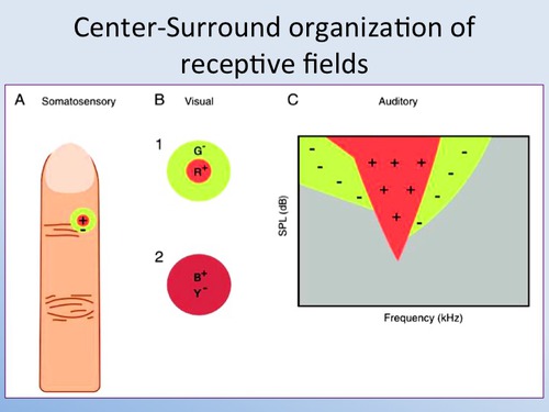
Рецептивные поля сенсорных нейронов имеют симметричную и антагонистическую структуру концентрических кругов. Ниже приводится несколько примеров из учебников по нейронауке.

http://thebrain.mcgill.ca/flash/d/d_02/d_02_cl/d_02_cl_vis/d_02_cl_vis.html

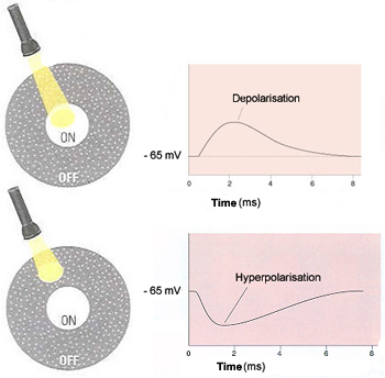
The receptive fields of bipolar cells are circular. But the centre and the surrounding area of each circle work in opposite ways: a ray of light that strikes the centre of the field has the opposite effect from one that strikes the area surrounding it (known as the "surround"). In fact, there are two types of bipolar cells, distinguished by the way they respond to light on the centers of their receptive fields. They are called ON-centre cells and OFF-centre cells. If a light stimulus applied to the centre of a bipolar cell's receptive field has an excitatory effect on that cell, causing it to become depolarized, it is an ON-centre cell. A ray of light that falls only on the surround, however, will have the opposite effect on such a cell, inhibiting (hyperpolarizing) it. 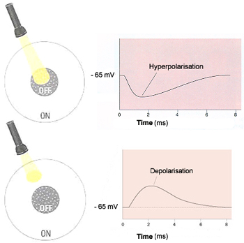The other kind of bipolar cells, OFF-centre cells, display exactly the reverse behavior: light on the field's centre has an inhibitory (hyperpolarizing) effect, while light on the surround has an excitatory (depolarizing ) effect. 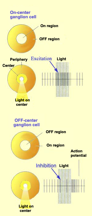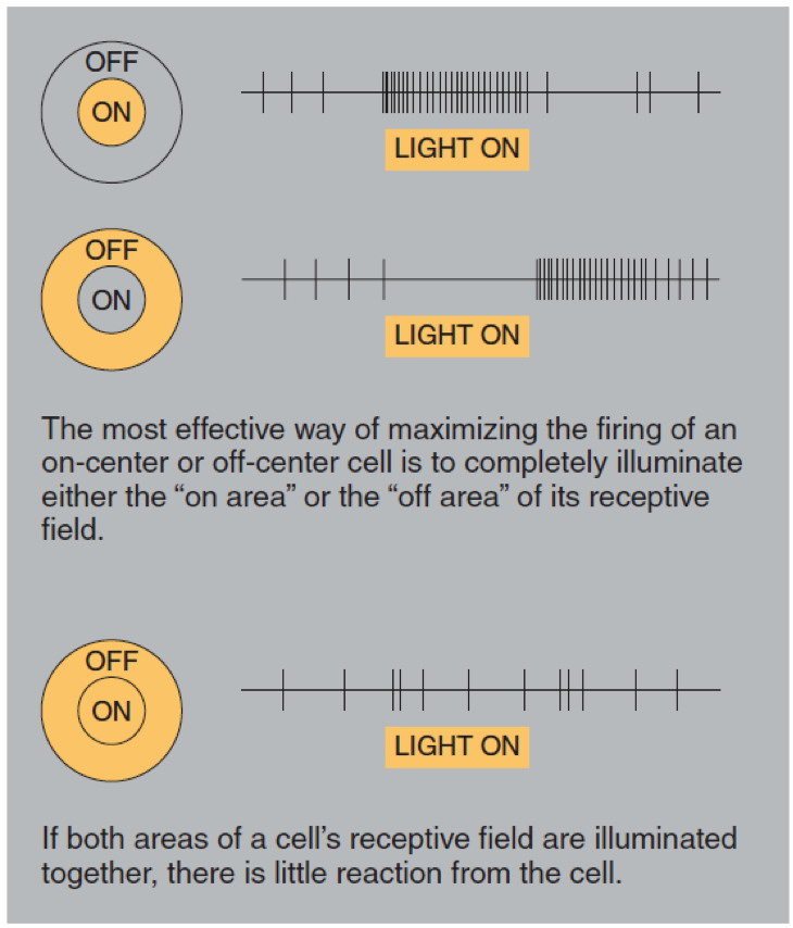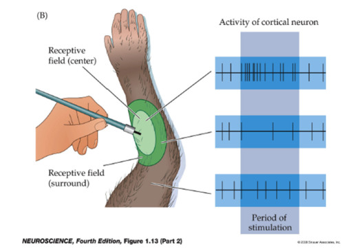Just like bipolar cells, ganglion cells have concentric receptive fields with a centre-surround antagonism. But contrary to the two types of bipolar cells, ON-centre ganglion cells and OFF-centre ganglion cells do not respond by depolarizing or hyperpolarizing, but rather by increasing or decreasing the frequency with which they discharge action potentials. That said, the response to the stimulation of the centre of the receptive field is always inhibited by the stimulation of the surround.

The Brain from Top to Bottom

http://mikeclaffey.com/psyc2/notes-vision.html

Notes: Vision (Part 1) PSYC 2: Biological Foundations - Fall 2012 - Professor Claffey

http://quizlet.com/4218195/7-somatosensory-system-flash-cards/

Quizlet. (7) Somatosensory System

http://quizlet.com/12718323/neuro-block3-flash-cards/

Quizlet. (7) Neuro ~ Block3

Ответная реакция реальных биологических нейронов на стимул

Ниже приводится несколько примеров данных экспериментальных измерений реальных биологических нейронов.

http://books.google.com/books?id=hkuVALWx_e4C&pg=PA172#v=onepage&q&f=false

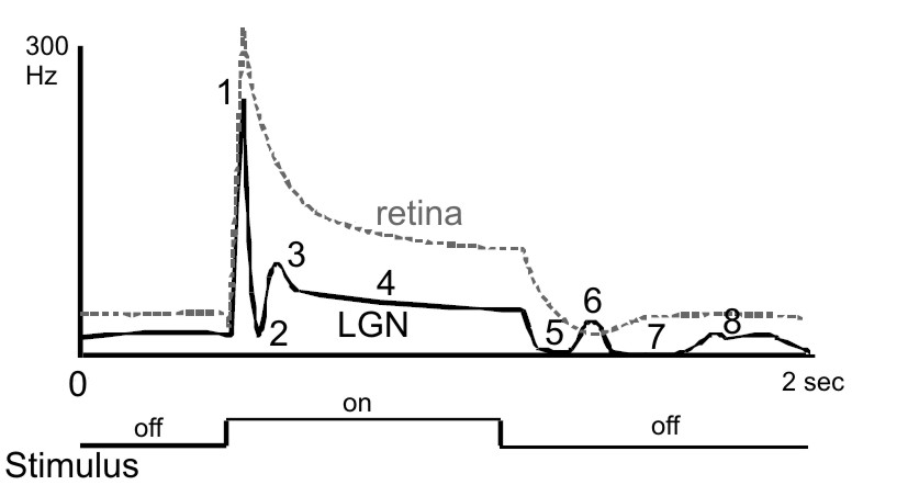
Figure 6. Typical LGN cell responses. The peri-stimulus-time histogram (PSTH) on top shows a typical temporal waveform of a geniculate (thick line) and retinal (broken line) visual response to a light spot flashed on and off within the center of the receptive field. The response to a sudden increment and decrement of RF illumination can show up to 8 components: 1) initial transient response (overshoot, peak), 2) post-peak inhibition, 3) early rebound response, 4) tonic response, 5) stimulus off inhibition (off-response), 6) first post-inhibitory rebound, 7) late inhibitory response, and 8) second post-inhibitory rebound. The response profile of the retinal input is less complex.

F Wörgötter, K Suder, N Pugeault, and K Funke (2003) Response characteristics in the lateral geniculate nucleus and their primary afferent influences on the visual cortex of cat Modulation of Neuronal Responses: Implications for Active Vision. (G T Buracas, O Ruksenas, G M Boyton and T D Albright, eds.) NATO Science Series 1: Life and Behavioral Sciences 334:165–188. Page 170

http://books.google.com/books?id=hkuVALWx_e4C&pg=PA170#v=onepage&q&f=false

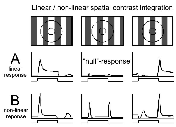
Figure 7. Linear, X-type (A) and nonlinear, Y-type (B) spatial contrast integration. A) The strongest visual responses of the linear type are elicited in LGN X-cells by a contrast pattern of a spatial frequency that fits well to the diameter of the center of the RF. The strength of the visual response depends on the spatial phase of the pattern (e.g. a grating). A balanced stimulation of the RF center (and surround) by bright and dark bars results in the null-response (middle) which is characterized by only small, if any, change in activity. B) Y-cell activity is more phasic and is also characterized by the lack of a null-response. Non-linear (second order) response peaks are observed irrespective of the spatial frequency of the stimulus.

F Wörgötter, K Suder, N Pugeault, and K Funke (2003) Response characteristics in the lateral geniculate nucleus and their primary afferent influences on the visual cortex of cat Modulation of Neuronal Responses: Implications for Active Vision. (G T Buracas, O Ruksenas, G M Boyton and T D Albright, eds.) NATO Science Series 1: Life and Behavioral Sciences 334:165–188. Page 172

http://books.google.com/books?id=hkuVALWx_e4C&pg=PA129#v=onepage&q&f=false

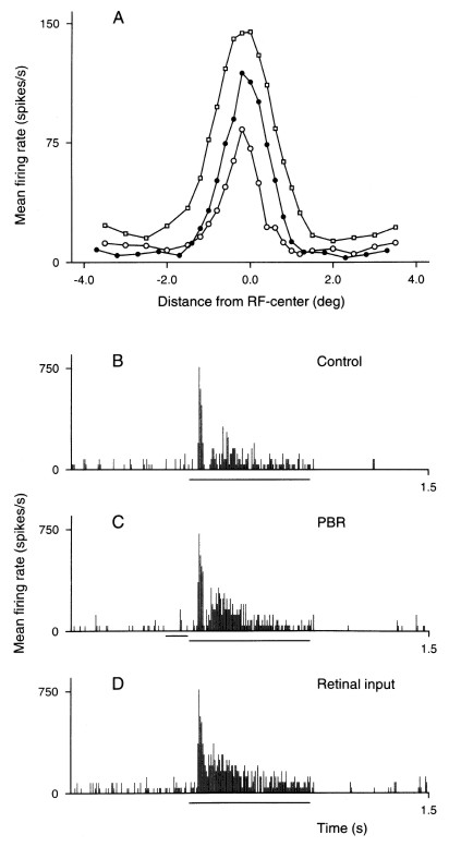
Figure 8. Effect of electrical PBR-stimulation on the spatial receptive field profile for an on-centre nonlagged Y-cell. A. Responses to a light slit presented in different position across the receptive field. The width of the slit was about 1/3 of the width of the handplotted receptive field centre, the slit length about 3 times the diameter of the hand-plotted receptive field centre. Each data point is the average of 5 stimulus presentations. Open circles, response of the dLGN cell in the control condition, open squares, retinal input measured by S-potentials. Filled spots, response of dLGN cell to electrical stimulation of PBR (140 Hz for 70 ms). B-D: Example of response patterns for the dLGN cell response in the control condition, with PBR-stimulation, and for the retinal input. The long horizontal line below the abcissa marks the period when the stimulus was on, the short bar marks the period with electrical PBR stimulation.

Paul Heggelund (2003) Signal Processing in the Dorsal Lateral Geniculate Nucleus Modulation of Neuronal Responses: Implications for Active Vision. (G T Buracas, O Ruksenas, G M Boyton and T D Albright, eds.) NATO Science Series 1: Life and Behavioral Sciences 334:109–134. Page 129

http://books.google.com/books?id=hkuVALWx_e4C&pg=PA119#v=onepage&q&f=false

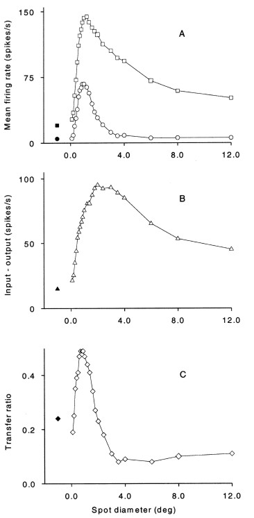
Figure 9. Comparison of the response of an on-centre X-cell and the response in its retinal input. The stimulus was a circular light spot of variable diameter but fixed contrast, centered on the receptive field. A. Open squares, retinal input, open circles, dLGN cell response. The response was measured as the average firing rate during a 500 ms period of spot presentation. Each point is the average from 20 stimulus presentations. Retinal input was measured as average frequency of S-potentials. The filled symbols mark spontaneous activity. B. The difference between retinal input and dLGN cell response. The data show the reduction in the average response to the various spot diameters. C. Transfer ratio calculated as output /input firing rate.

Paul Heggelund (2003) Signal Processing in the Dorsal Lateral Geniculate Nucleus Modulation of Neuronal Responses: Implications for Active Vision. (G T Buracas, O Ruksenas, G M Boyton and T D Albright, eds.) NATO Science Series 1: Life and Behavioral Sciences 334:109–134. Page 119

Дополнительное чтение

Нейрокластерная Модель Мозга

«Нейромодель RF-PSTH» и «Нейрокластерная Модель Мозга» – это две разные, не связанные между собой модели.
Истинность или ошибочность «Нейромодели RF-PSTH» никак не связанна с истинностью или ошибочностью «Нейрокластерной Модели Мозга».

Электронная почта для связи:
info@neuroclusterbrain.com

© 2020 neuroclusterbrain.com. Онлайн с 11 июля 2013