Free teaching tool for
students, teachers and scientists of
neuroscience, biophysics, biomedical engineering and artificial
intelligence.
Abstract
Currently available artificial neuron models are unable
to simulate fundamentally important features of real biological
neurons: 1) antagonistic receptive fields and 2) PSTH output signal of
neuron to any stimulus.
Even if some neuron models try to simulate antagonistic receptive
fields then they are unable to simulate PSTH output signal, and vice
versa – some other models try to simulate PSTH output signal of neuron,
however these models fail to explain antagonistic receptive fields of
neurons.
As for example, a very popular DOG (Difference Of Gaussians) model
simulates antagonistic structure of the receptive field, however DOG
model fails to simulate PSTH output signal of neuron. And the vast
majority of artificial neural models even fail to simulate both:
antagonistic receptive fields and PSTH output signal.
For the first time ever neuron model RF-PSTH is able to simulate both
antagonistic receptive fields and PSTH output signal.
Neuron model RF-PSTH is based on physics of real biological neurons.
Recommended literature
Comprehensive description of the receptive field of biological neuron
is available in the book “Encyclopedia
of the Human Brain” written by Vilayanur S. Ramachandran MBBS PhD
Hon. FRCP (Editor), published by Academic Press in July 10, 2002 (1
edition), ISBN-10: 0122272102, ISBN-13: 978-0122272103.
In this book please read Chapter “Receptive Field” written by Rajesh P.
N. Rao (University of Washington), in pages 155-168.
Neuron model RF-PSTH simulates neuron’s features described in this
Chapter.
The importance and advantage of new neuron model RF-PSTH
Output PSTH signal produced by neuron model RF-PSTH matches
experimental measurements of real biological neurons in laboratory.
Measurements of real biological neurons show that receptive fields of
sensory neurons have symmetrical concentric antagonistic
circular structure, however current science does not have any
convincing explanation what is the cause of this phenomenon. It is
hypothesized that antagonistic concentric receptive fields are formed
because neuron connects to receptors (or to other neurons) via synaptic
connections and supposedly these synaptic connections are distributed
in such a way that concentric antagonistic circles are formed. There is
no convincing explanation why receptive fields should form concentric
antagonistic circular structures.
Neuron model RF-PSTH is able to simulate concentric antagonistic
circular structures of the receptive fields of sensory neurons.
Neuron model RF-PSTH claims that antagonistic circular structure of the
receptive field is the internal feature of all sensory neurons,
and there is no need for any external neural links (external neural
networks) in order to form such antagonistic circular structures.
Neuron model RF-PSTH program
Download “Neuron model RF-PSTH” v.2.5 native applications for the
following platforms:
Neuron model RF-PSTH program is free to use for academic and
educational purposes.
Description of neuron model RF-PSTH
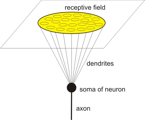
Neuron possesses a cell body (soma), dendrites, and an axon.
Neuron is modeled as 3D object in 3D space:
1) the soma of neuron is modeled as mathematical point;
2) the receptive field of neuron is modeled as two dimensional plane;
3) from soma of neuron the dendrites reach two dimensional plane;
4) in two dimensional plane dendrites form circular receptive field;
5) 3D shape of neuron is the right circular cone in which the apex of
the cone represents neuron soma and the base of the cone represents
receptive field.
A good example for such scenario is the ganglion (neural)
cell which receives the input from photoreceptors in the retina. Many
other neurons also fit into this scenario quite well, as for example
somatosensory neurons which receive input from receptors on the skin,
etc.
Figure
1. Neuron is modeled as
3D object in 3D space
Neuron model RF-PSTH claims that if all these above mentioned
conditions are fulfilled then the neuron will have symmetrical
concentric antagonistic circular structure of the receptive field.
However if the receptive field of neuron will have another
configuration (like for example will be the part of 3D sphere or will
have some other configuration) then neuron’s receptive field might be
without concentric antagonistic circular structure. In other words, 3D
spatial configuration of the neuron plays essential role in the
formation of receptive field structure.
FAQ (Frequently Asked Questions)
about neuron model RF-PSTH
Receptive fields of neurons can have more complicated structure
than concentric antagonistic circles, as for example receptive fields
of V1 neurons are lines, bars or squared shapes inclined at certain
degree and so on, however neuron model RF-PSTH does not model such
complicated
receptive fields of the neuron thus I think that neuron model RF-PSTH
is a bad/incomplete model, isn’t it?
We get this question repeatedly over and over again even from people
who have high academic degrees in neuroscience so here is the answer.
First of all, “receptive field of V1 neuron” (as shown in neuroscience
textbooks and articles) has a misleading name – actually it is not the
receptive field of the single neuron, it is the receptive field of
multilayer network (from retina through LGN into V1). However
multilayer network and single neuron are two different things. Neuron
model RF-PSTH models the behavior of the single neuron, not the
behavior of multilayer network. If you will take out truly single V1
neuron (throwing away all neighboring neurons) and if you will measure
the input-output characteristics of truly single V1 neuron then you
will get the same results as in neuron model RF-PSTH. In other words,
the major misunderstanding comes from confusing the receptive field of
the single
neuron with the receptive field of multilayer network.
Which types of neurons of which part of the brain (cerebral
cortex, thalamus, hypothalamus, amygdala, hippocampus, etc) does the
neuron model RF-PSTH simulate?
Neuron model RF-PSTH simulates neurons which have spatial 3D shape of
right circular cone (as shown in Figure 1). It does matter in which
part of the brain such neuron is located, as long as it will have
spatial 3D shape of right circular cone, the neuron model RF-PSTH will
simulate behavior of such neuron. However in practice the neurons of
right circular cone shape are most easily found in the first layer of
multiple sensory modality inputs, a good example for such scenario is
the ganglion (neural) cell which receives the input from photoreceptors
in the retina, many other neurons also fit into this scenario quite
well, as for example somatosensory neurons which receive input from
receptors on the skin, etc.
Neuron model RF-PSTH supports the hypothesis of Vernon Benjamin
Mountcastle (Professor Emeritus of Neuroscience at Johns Hopkins
University) who noticed that different areas of neocortex (visual,
auditory, etc) are remarkably uniform in appearance and structure and
proposed the idea that different areas of neocortex process information
performing the same basic operation.
Vernon Benjamin Mountcastle
(July 15, 1918 – January 11, 2015) was Professor Emeritus of
Neuroscience at Johns Hopkins University. He discovered and
characterized the columnar organization of the cerebral cortex in the
1950s. This discovery was a turning point in investigations of the
cerebral cortex, as nearly all cortical studies of sensory function
after Mountcastle's 1957 paper, on the somatosensory cortex, used
columnar organization as their basis.
Wikipedia
Chapter: An
Organizing Principle for Cerebral Function: The Unit Model and the
Distributed System
By Vernon B.
Mountcastle
Excerpt from pages 39-40:
<....>
Functional Properties of Distributed Systems
It is well known from classical neuroanatomy that many of the large
entities of the brain are interconnected by extrinsic pathways into
complex systems, including massive reentrant circuits. Three sets of
recent discoveries, described above, have put the systematic
organization of the brain in a new light. The first is that many of the
major structures of the brain are constructed by replication of
identical multicellular units. These modules are local neural circuits
of hundreds or thousands of cells linked together by a complex
intramodular connectivity. The modules of any one entity are more or
less similar throughout, but those of different entities may differ
strikingly. The modular unit of the neocortex is the vertically
organized group of cells I have described earlier. These basic units
are single translaminar cords of neurons, the minicolumns, which in
some areas are packaged into larger processing units whose size and
form appear to differ from one place to another. Nevertheless, the
qualitative nature of the processing function of the neocortex is
thought to be similar in different areas, though that intrinsic
processing apparatus may be subject to modification as a result of past
history, particularly during critical periods in ontogenetic
development.
The Mindful Brain
By Gerald M. Edelman and Vernon B.
Mountcastle, eds.
MIT Press. 1978. ISBN-10: 026205020X. ISBN-13: 978-0262050203.
Step-by-step instructions how to run neuron model RF-PSTH
Step #1
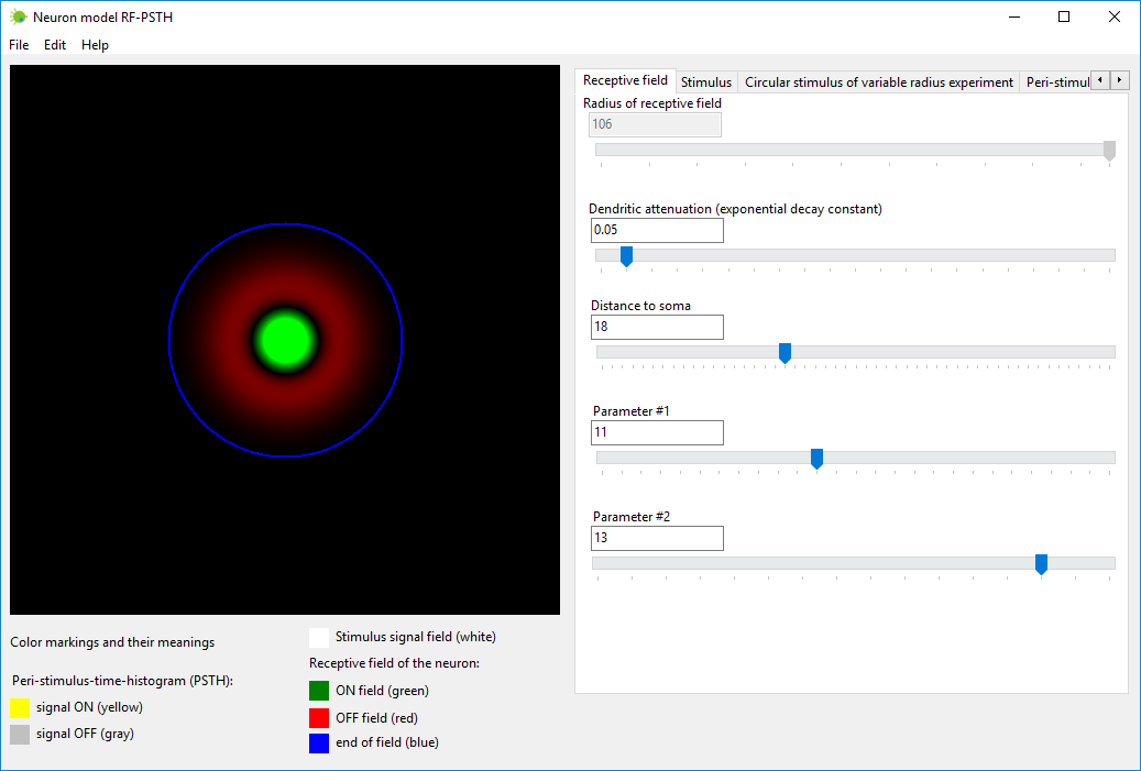
Set the parameters which determine the structure of receptive field of
neuron. This can be accomplished in tab named “Receptive field”.
The parameters of neuron are the following: Radius of receptive field – this parameter calculated
automatically, you do not need to set this parameter; Dendritic attenuation (exponential decay constant) – when signal
travels via dendrites, the signal attenuates according to exponential
decay law,
this parameter sets exponential decay constant; Distance to soma – distance from soma to the receptive field
plane; Parameter #1 – parameter related to the diameter of dendrites; Parameter #2 – one more neuron parameter.
Figure 2. Tab “Receptive field” in neuron model RF-PSTH.
The receptive field of a sensory
neuron is a region of space in which the presence of a
stimulus will alter the firing of that neuron. Receptive fields have
been identified for neurons of the auditory system, the somatosensory
system, and the visual system.
The concept of receptive fields can be extended to further up the
neural system; if many sensory receptors all form synapses with a
single cell further up, they collectively form the receptive field of
that cell. For example,
the receptive field of a ganglion cell in the retina of the eye is
composed
of input from all of the photoreceptors which synapse with it, and a
group of ganglion cells in turn forms the receptive field for a cell in
the
brain. This process is called convergence.
<...>
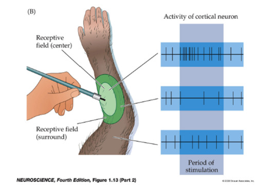
On center and off center retinal ganglion cells respond oppositely to
light in the center and surround of their receptive fields. A strong
response means high frequency firing, a weak response is firing at a
low frequency, and no response means no action potential is fired.
Wikipedia
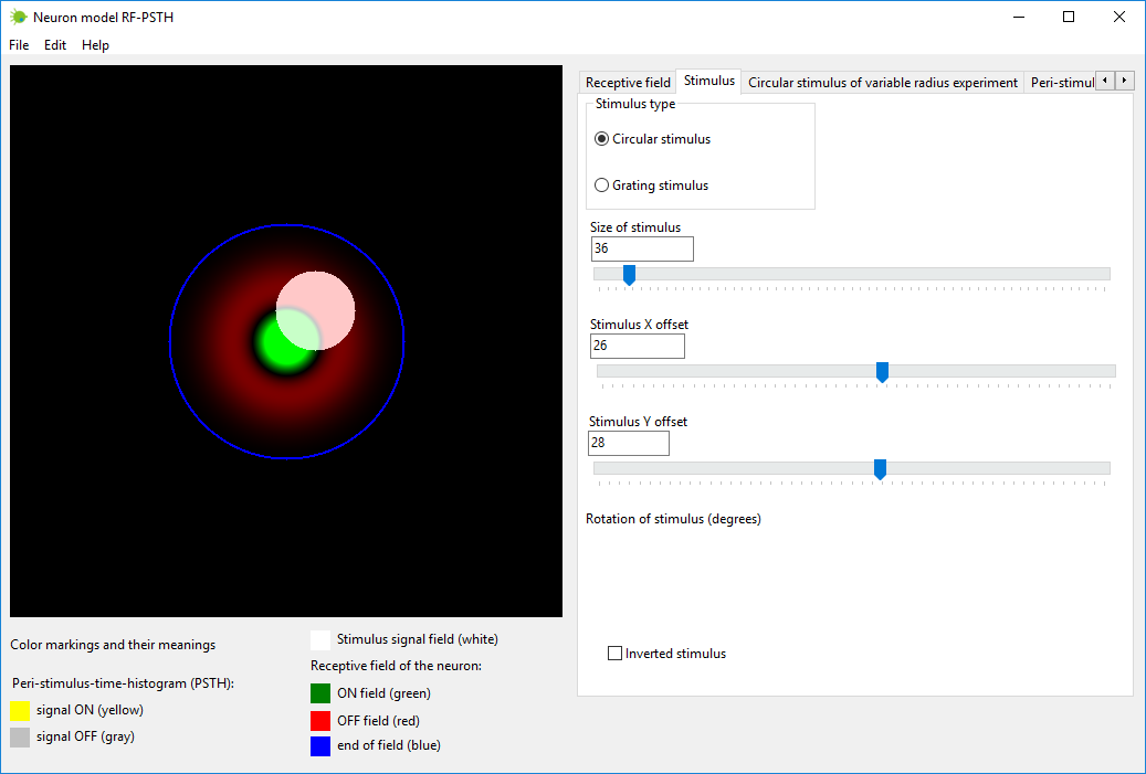
Step #2
Create the stimulus with the parameters needed. This can be
accomplished in tab named “Stimulus”.
Stimulus is painted with white color over the receptive field of the
neuron.
Stimulus can be of several types:
1) circular stimulus – you can
change the radius of the circle and coordinates
(x, y);
2) grating stimulus – you can
change the width of the grating, translation
coordinates (x, y), and rotation angle (in degrees);
3) inverted stimulus – inverts
stimulated and non-stimulated areas.
Circular stimulus can be manipulated directly with mouse (resized and
moved) by clicking with mouse on stimulus image.
Grating stimulus can be manipulated only by sliding trackbars.
Neuron model RF-PSTH also allows to simulate reaction of neuron to the
moving stimulus, however this program provides the ability to simulate
only static
non-moving stimulus.
In physiology, a stimulus
(plural stimuli) is a detectable change in the internal or external
environment. The ability of an organism or organ to respond to external
stimuli is called sensitivity.
When a stimulus is applied to a sensory receptor, it normally elicits
or
influences a reflex via stimulus transduction. These sensory receptors
can receive
information from outside the body, as in touch receptors found in the
skin or light
receptors in the eye, as well as from inside the body, as in
chemoreceptors and mechanorceptors.
Wikipedia
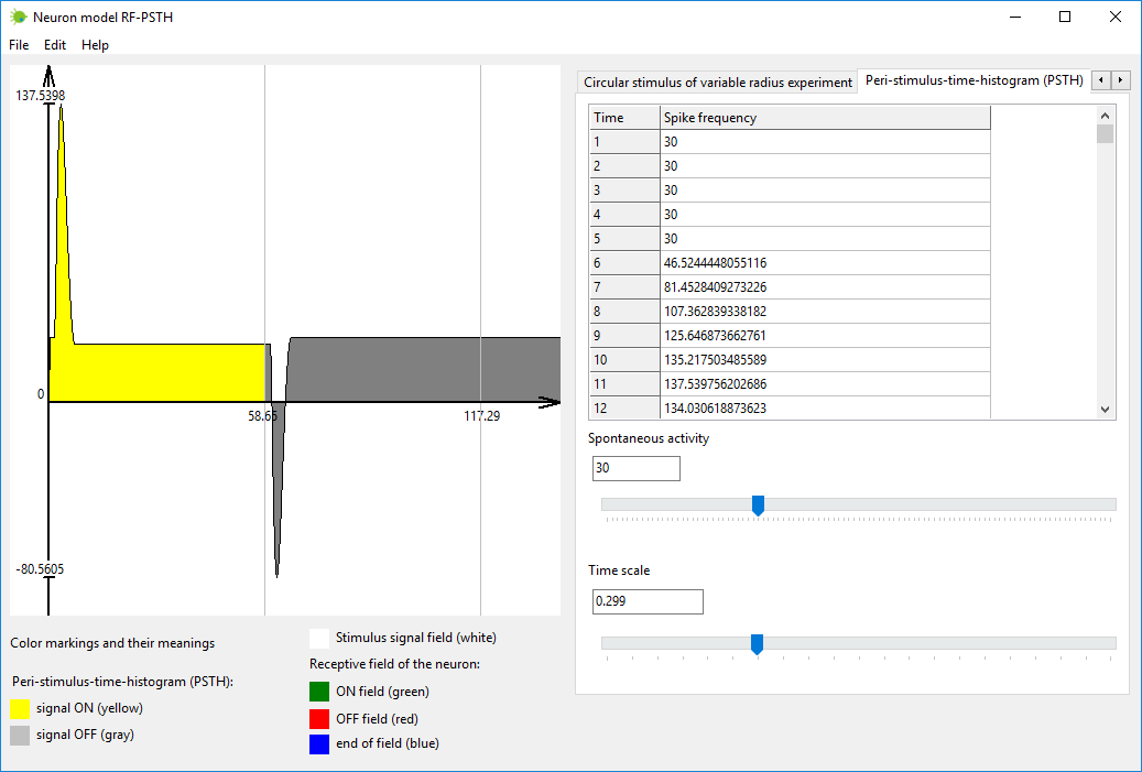
Step #3
Simulate neuron output signal as the reaction to input stimulus. This
can be accomplished in tab named “Peri-stimulus-time-histogram (PSTH)”.
Stimulus is turned on when time is zero. Stimulus is turned off
automatically, when neuron output signal stabilizes and becomes almost
stationary.
Neuron output is painted yellow when stimulus is on, and painted gray
when stimulus is off.
Figure 4. Tab “Peri-stimulus-time-histogram (PSTH)” in neuron model
RF-PSTH.
In neurophysiology, peristimulus
time histogram and poststimulus time histogram, both abbreviated PSTH
or PST histogram, are histograms of the times at which neurons fire.
These histograms are used to visualize the rate and timing of neuronal
spike discharges in relation to an
external stimulus or event. The peristimulus time histogram is
sometimes called perievent
time histogram, and post-stimulus and peri-stimulus are often
hyphenated.
The prefix peri, for through, is typically used in the case of periodic
stimuli, in which case the PSTH show neuron firing times wrapped to one
cycle of the stimulus.
The prefix post is used when the PSTH shows the timing of neuron
firings in response to a stimulus event or onset.
To make a PSTH, a spike train recorded from a single neuron is aligned
with the onset, or a fixed phase point, of an identical stimulus
repeatedly presented to an animal. The aligned sequences are
superimposed in time,
and then used to construct a histogram.
Wikipedia
Additional notes about PSTH output
Real biological neurons cannot produce negative frequency of spikes in
the output. However this negative output signal can be measured as
reduced presynaptic potential inside neuron soma in place where axon
connects to soma. The simulation program shows and reveals internal
processes in the neuron.
PSTH output is calculated without short-term depression (STD) and
short-term facilitation (STF).
Short-term
plasticity (STP), also called dynamical synapses, refers to a
phenomenon in which synaptic efficacy changes over time in a way that
reflects the history of presynaptic activity. Two types of STP, with
opposite effects on synaptic efficacy, have been observed in
experiments. They are known as short-term depression (STD) and
short-term facilitation (STF). STD is caused by depletion of
neurotransmitters consumed during the synaptic signaling process at the
axon terminal of a pre-synaptic neuron, whereas STF is caused by influx
of calcium into the axon terminal after spike generation, which
increases the release probability of neurotransmitters. STP has been
found in various cortical regions and exhibits great diversity in
properties. Synapses in different cortical areas can have varied forms
of plasticity, being either STD-dominated, STF-dominated, or showing a
mixture of both forms.
Compared with long-term plasticity, which is hypothesized as the neural
substrate for experience-dependent modification of neural circuit, STP
has a shorter time scale, typically on the order of hundreds to
thousands of milliseconds. The modification it induces to synaptic
efficacy is temporary. Without continued presynaptic activity, the
synaptic efficacy will quickly return to its baseline level.
Scholarpedia
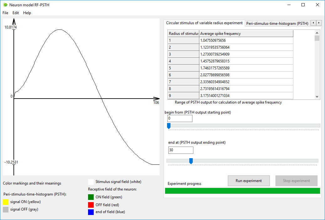
Step #4
Simulate circular stimulus of variable radius experiment. This can be
accomplished in tab named “Circular stimulus of variable radius
experiment”.
The description of experiment is following. Circular stimulus is placed
in the center of the receptive field. The size of stimulus is increased
in steps of one, starting from zero till the size of the receptive
field. In each step PSTH output signal is calculated. In each step a
range of output values from PSTH graph are taken and the average spike
frequency for that defined range is calculated. The final produced
graph of the experiment is the average spike frequency dependency from
the stimulus size. The form of final produced graph is sensitive on the
selected range from PSTH output signal from which average spike
frequency is calculated. The changing of the selected range (of PSTH
output signal) changes the graph of final experiment graph. There are
no rules in neuroscience which define which exactly range of PSTH
signal should be taken for average spike frequency calculation, thus
you need to experiment with the range values yourself in order to find
out which range better suits your needs.
Figure 5. Tab “Circular stimulus of variable radius experiment” in
neuron model RF-PSTH.
The flaws of currently available artificial neuron models and
the superiority of neuron model RF-PSTH
Mathematical modeling of any physical phenomenon requires
simplifications (reductions) of the phenomenon in order to decrease the
number of parameters and to reduce the number of calculations.
The technical question is how much the phenomenon can be simplified
(reduced) in order not to loose essential information which is needed
for solving of the particular problem.
As for example, when we need to analyze a car driving on the road, we
can simplify the car into mathematical point (without dimension and
without mass) which moves across two dimensional space with some speed.
Such simplified car model is perfectly good when we want to calculate,
for example, how much time it will take to drive a car from point A to
point B. However, if we want to find out what force is applied to brake
plates of the car when the driver pushes the brake pedal in order to
stop the car, then a model in which the car is represented as
mathematical point will be insufficient to solve such problem. If you
want to find out what force is applied to brake plates of the car when
the driver pushes the brake pedal then you need to know the mass of the
car, the diameter of the wheels, etc – however all these parameters
were eliminated in the car model described above. In other words, when
mathematical model is created, some essential features (parameters) can
be eliminated, without which it will be impossible to solve some
special practical problems.
Let’s look more closely what artificial neuron models are used today.
The first artificial neuron was the Threshold Logic Unit (TLU) first
proposed by Warren McCulloch and Walter Pitts in 1943. As a transfer
function, it employed a threshold, equivalent to using the Heaviside
step function. Initially, only a simple model was considered, with
binary inputs and outputs, some restrictions on the possible weights,
and a more flexible threshold value. Since the beginning it was already
noticed that any boolean function could be implemented by networks of
such devices, what is easily seen from the fact that one can implement
the AND and OR functions, and use them in the disjunctive or the
conjunctive normal form.
Researchers also soon realized that cyclic networks, with feedbacks
through neurons, could define dynamical systems with memory, but most
of the research concentrated (and still does) on strictly feed-forward
networks because of the smaller difficulty they present.
One important and pioneering artificial neural network that used the
linear threshold function was the perceptron, developed by Frank
Rosenblatt. This model already considered more flexible weight values
in the neurons, and was used in machines with adaptive capabilities.
The representation of the threshold values as a bias term was
introduced by Bernard Widrow in 1960.
In the late 1980s, when research on neural networks regained strength,
neurons with more continuous shapes started to be considered. The
possibility of differentiating the activation function allows the
direct use of the gradient descent and other optimization algorithms
for the adjustment of the weights. Neural networks also started to be
used as a general function approximation model.
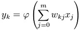
<...> Basic structure
For a given artificial neuron, let there be m + 1 inputs with signals x0
through xm and weights w0 through wm.
Usually, the x0 input is assigned the value +1,
which makes it a bias input with wk0 = bk.
This leaves only m actual
inputs to the neuron: from x1 to xm.
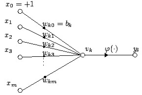
The output of kth neuron is:
Where φ is the transfer
function.
The output is analogous to the axon of a biological neuron, and its
value propagates to input of the next layer, through a synapse. It may
also exit the system, possibly as part of an output vector.
It has no learning process as such. Its transfer function weights are
calculated and threshold value are predetermined.
<...> Types of transfer functions
The transfer function of a neuron is chosen to have a number of
properties which either enhance or simplify the network containing the
neuron. Crucially, for instance, any multilayer perceptron using a
linear transfer function has an equivalent single-layer network; a
non-linear function is therefore necessary to gain the advantages of a
multi-layer network.
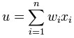
Below, u refers in all cases to the weighted sum of all the inputs to
the neuron, i.e. for n inputs,
where w is a vector of
synaptic weights and x is a
vector of inputs.
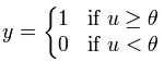
Step function
The output y of this transfer function is binary, depending on whether
the input meets a specified threshold, θ. The "signal" is sent, i.e. the
output is set to one, if the activation meets the threshold.
This function is used in perceptrons and often shows up in many other
models. It performs a division of the space of inputs by a hyperplane.
It is specially useful in the last layer of a network intended to
perform binary classification of the inputs. It can be approximated
from other sigmoidal functions by assigning large values to the weights.
Linear combination
In this case, the output unit is simply the weighted sum of its inputs
plus a bias term. A number of such linear neurons perform a linear
transformation of the input vector. This is usually more useful in the
first layers of a network. A number of analysis tools exist based on
linear models, such as harmonic analysis, and they can all be used in
neural networks with this linear neuron. The bias term allows us to
make affine transformations to the data.
Sigmoid
A fairly simple non-linear function, a Sigmoid function such as the
logistic function also has an easily calculated derivative, which can
be important when calculating the weight updates in the network. It
thus makes the network more easily manipulable mathematically, and was
attractive to early computer scientists who needed to minimize the
computational load of their simulations. It is commonly seen in
multilayer perceptrons using a backpropagation algorithm.
<...> Comparison to biological neurons
Artificial neurons bear a striking similarity to their biological
counterparts.
Dendrites - In a biological neuron, the dendrites act as the input
vector. These dendrites allow the cell to receive signals from a large
(>1000) number of neighboring neurons. As in the above mathematical
treatment, each dendrite is able to perform "multiplication" by that
dendrite's "weight value." The multiplication is accomplished by
increasing or decreasing the ratio of synaptic neurotransmitters to
signal chemicals introduced into the dendrite in response to the
synaptic neurotransmitter. A negative multiplication effect can be
achieved by transmitting signal inhibitors (i.e. oppositely charged
ions) along the dendrite in response to the reception of synaptic
neurotransmitters.
Soma - In a biological neuron, the soma acts as the summation function,
seen in the above mathematical description. As positive and negative
signals (exciting and inhibiting, respectively) arrive in the soma from
the dendrites, the positive and negative ions are effectively added in
summation, by simple virtue of being mixed together in the solution
inside the cell's body.
Axon - The axon gets its signal from the summation behavior which
occurs inside the soma. The opening to the axon essentially samples the
electrical potential of the solution inside the soma. Once the soma
reaches a certain potential, the axon will transmit an all-in signal
pulse down its length. In this regard, the axon behaves as the ability
for us to connect our artificial neuron to other artificial neurons.
Unlike most artificial neurons, however, biological neurons fire in
discrete pulses. Each time the electrical potential inside the soma
reaches a certain threshold, a pulse is transmitted down the axon. This
pulsing can be translated into continuous values. The rate (activations
per second, etc.) at which an axon fires converts directly into the
rate at which neighboring cells get signal ions introduced into them.
The faster a biological neuron fires, the faster nearby neurons
accumulate electrical potential (or lose electrical potential,
depending on the "weighting" of the dendrite that connects to the
neuron that fired). It is this conversion that allows computer
scientists and mathematicians to simulate biological neural networks
using artificial neurons which can output distinct values (often from
-1 to 1).
Wikipedia
All these artificial neuron models are unable to explain and to
simulate antagonistic receptive fields and PSTH output signal of real
biological neurons.
Artificial Neural Networks are built using such incapable artificial
neurons.
If Artificial Neural Network (ANN) is built from neurons with linear
transfer function then such multilayer network can be simplified into
single-layer network which will be equivalent to original multilayer
network. A nonlinear transfer function is therefore necessary in order
to gain advantages of a multilayer network.
We have noted before that if we have a regression problem with
non-binary network outputs, then it is appropriate to have a linear
output activation function. So why not simply use linear activation
functions on the hidden layers as well?
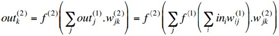
With activation functions f(n)(x)
at layer n, the outputs of a
two-layer MLP are
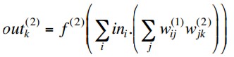
so if the hidden layer activations are linear, i.e. f(1)(x) = x, this simplifies to
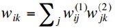
But this is equivalent to a single layer network with weights
and we know that such a network cannot deal with non-linearly separable
problems.
Learning in Multi-Layer
Perceptrons - Back-Propagation
Neural Computation : Lecture 7
John A. Bullinaria, 2013
If artificial neuron will be built using linear transfer function
and
if the number of neuron inputs will be reduced to one(1) input then
information processing capabilities of such neuron will drop almost to
zero. This example clearly shows that oversimplification of real
physical object will render mathematical model incapable of solving
practical problems.
Computer scientists who work with artificial neural networks prefer to
use:
1) neurons with nonlinear transfer function believing that nonlinear
perceptron is superior to linear perceptron;
2) multilayer networks with nonlinear transfer function because it was
proved that single-layer network could not be trained to recognize many
classes of patterns.
The perceptron algorithm was
invented in 1957 at the Cornell Aeronautical Laboratory by Frank
Rosenblatt.
<...>
Although the perceptron initially seemed promising, it was eventually
proved that perceptrons could not be trained to recognize many classes
of patterns. This led to the field of neural network research
stagnating for many years, before it was recognised that a feedforward
neural network with two or more layers (also called a multilayer
perceptron) had far greater processing power than perceptrons with one
layer (also called a single layer perceptron). Single layer perceptrons
are only capable of learning linearly separable patterns; in 1969 a
famous book entitled Perceptrons by Marvin Minsky and Seymour Papert
showed that it was impossible for these classes of network to learn an
XOR function. It is often believed that they also conjectured
(incorrectly) that a similar result would hold for a multi-layer
perceptron network. However, this is not true, as both Minsky and
Papert already knew that multi-layer perceptrons were capable of
producing an XOR Function. <...> Three years later Stephen
Grossberg published a series of papers introducing networks capable of
modelling differential, contrast-enhancing and XOR functions. (The
papers were published in 1972 and 1973, see e.g.: Grossberg, Contour
enhancement, short-term memory, and constancies in reverberating neural
networks. Studies in Applied Mathematics, 52 (1973), 213-257, online).
Nevertheless the often-miscited Minsky/Papert text caused a significant
decline in interest and funding of neural network research. It took ten
more years until neural network research experienced a resurgence in
the 1980s. This text was reprinted in 1987 as "Perceptrons - Expanded
Edition" where some errors in the original text are shown and corrected.
The kernel perceptron algorithm was already introduced in 1964 by
Aizerman et al. Margin bounds guarantees were given for the Perceptron
algorithm in the general non-separable case first by Freund and
Schapire (1998), and more recently by Mohri and Rostamizadeh (2013) who
extend previous results and give new L1 bounds.
Wikipedia
Computer scientists fail to notice one key fundamental feature of
the perceptron – when perceptron is used for pattern recognition tasks
the
perceptron acts as a simple template matching technique and it does not
matter if the transfer function of the perceptron is linear or
nonlinear, nonlinearity does not help at all – the perceptron acts as
simple template matching technique. And it is well known fact that
template matching technique fails to recognize object when object is
resized, rotated or moved. In other words, computer scientists fail to
notice the obvious fact that perceptron is fundamentally unable to
recognize object which is transformed (resized, rotated or moved).
When backpropagation training technique is used to train nonlinear
perceptron to filter out audio signal then experimental results show
that when the number of training iterations approach to the infinity
then the weights of perceptron approach the coefficients of DSP filter
which is optimal to filter out that particular signal. In other words,
it does not matter if the transfer function of the perceptron is
linear or nonlinear – the perceptron acts as a simple linear DSP
filter. The nonlinearity of the perceptron’s transfer function does not
provide any advantage over linear DSP filter.
Computer scientists who work with artificial neural networks use
oversimplified mathematical models of the neuron which are incapable to
solve practical pattern recognition problems. When artificial neuron
was invented it was claimed that soon mankind will have the machines
which are able to solve the same pattern recognition tasks as the
biological brain is able to solve. However, despite the decades of
research and tedious work, the nonlinear multilayer perceptrons are
still incapable to solve even most primitive pattern recognition tasks.
The reason of such failure is obvious – the models of artificial neuron
are oversimplified and lack some essential features of real biological
neuron. As for example these neuron models lack antagonistic receptive
field structure, etc.
As a rule, computer scientists don’t even know what the thing
“receptive field” is and their knowledge about features and parameters
of real biological neurons is almost zero - they do not know that
receptive fields of sensory neurons have symmetrical concentric
antagonistic circular structure and so on.
Neuron model RF-PSTH overcomes the flaws and limitations of current
artificial neuron models.
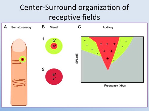
Receptive field structure of real biological neurons
Receptive fields of sensory neurons have symmetrical concentric
antagonistic circular structure. Several examples from neuroscience
textbooks are provided below.
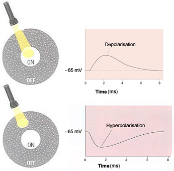
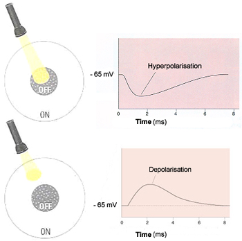
The receptive fields of bipolar
cells are circular. But the centre and the
surrounding area of each circle work in opposite ways: a ray of light
that strikes the centre of the field has the opposite effect from one
that strikes the area surrounding it (known as the "surround").
In fact, there are two types of bipolar cells, distinguished by the way
they respond to light on the centers of their receptive fields. They
are called ON-centre cells and OFF-centre cells.
If a light stimulus applied to the centre of a bipolar cell's
receptive field has an excitatory effect on that cell, causing it to
become depolarized, it is an ON-centre cell. A ray of light that falls
only on the surround, however, will have the opposite effect on such a
cell, inhibiting (hyperpolarizing) it.
The other kind of bipolar cells, OFF-centre cells,
display exactly the reverse behavior: light on the field's centre has
an inhibitory (hyperpolarizing) effect, while light on the surround has
an excitatory (depolarizing ) effect.
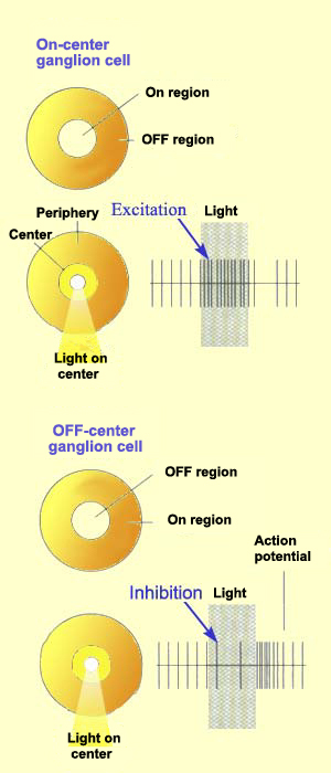
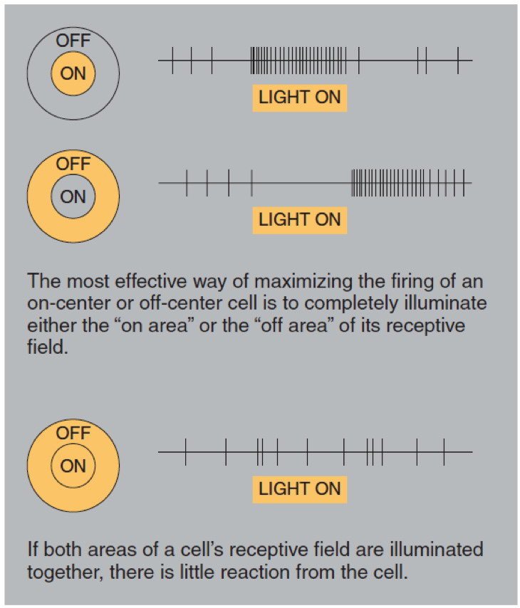
Just like bipolar cells, ganglion cells have concentric receptive
fields with a centre-surround antagonism. But contrary to the two types
of bipolar cells, ON-centre ganglion cells and OFF-centre ganglion
cells do not respond by depolarizing or hyperpolarizing, but rather by
increasing or decreasing the frequency with which they discharge action
potentials.
That said, the response to the stimulation of the centre of the
receptive field is always inhibited by the stimulation of the surround.
Olfactory and Gustatory
Receptive Fields
<...>
olfactory receptive fields are analogous to retinal center-surround
receptive fields: Mitral cells in the olfactory bulb exhibit excitatory
responses to certain chemical compounds in a homologous series of
compounds and inhibitory responses to neighboring compounds that flank
the excitatory compounds in the series. The presence of antagonistic
center-surround receptive fields in the olfactory system suggests that
higher level receptive fields, such as those of neurons in the
olfactory cortex, may possess an oriented structure analogous to visual
and auditory cortical receptive fields. However, the orientation would
be in the space of chemical concentration and time, implying a
sensitivity toward increasing or decreasing amounts of particular
chemical compounds at a particular rate.
Encyclopedia of The Human Brain
- Vol. I, II, III and IV (2002). Editor-in-Chief: V. S. Ramachandran.
ISBN: 978-0-12-227210-3.
Volume IV, Page 165
On-center and
Off-center receptive fields. The receptive fields of retinal ganglion
cells and thalamic neurons are
organized as two concentric circles with different contrast polarities.
On-center neurons respond to the presentation of a light spot on a dark
background and off-center
neurons to the presentation of a dark spot on a light background.
Scholarpedia
Output response of real biological neurons to the stimulus
Below are several examples of experimental measurement data of real
biological neurons.
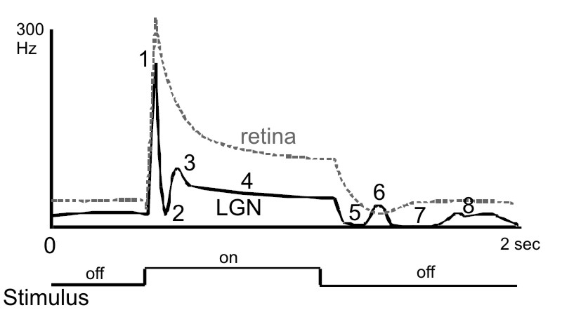
Figure 6. Typical LGN cell responses. The peri-stimulus-time histogram
(PSTH) on top shows a typical temporal waveform of a geniculate (thick
line) and retinal (broken line) visual response to a light spot flashed
on and off within the center of the receptive field. The response to a
sudden increment and decrement of RF illumination can show up to 8
components: 1) initial transient response (overshoot, peak), 2)
post-peak inhibition, 3) early rebound response, 4) tonic response, 5)
stimulus off inhibition (off-response), 6) first post-inhibitory
rebound, 7) late inhibitory response, and 8) second post-inhibitory
rebound. The response profile of the retinal input is less complex.
F Wörgötter, K Suder, N
Pugeault, and K Funke (2003)
Response characteristics in the lateral geniculate nucleus and their
primary afferent influences on the visual cortex of cat
Modulation of Neuronal Responses: Implications for Active Vision. (G T
Buracas, O Ruksenas, G M Boyton and T D Albright, eds.) NATO Science
Series 1: Life and Behavioral Sciences 334:165–188.
Page 170
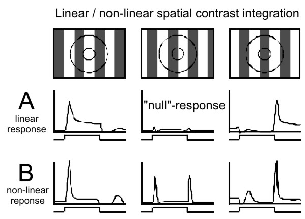
Figure 7. Linear, X-type (A) and nonlinear, Y-type (B) spatial contrast
integration. A) The strongest visual responses of the linear type are
elicited in LGN X-cells by a contrast pattern of a spatial frequency
that fits well to the diameter of the center of the RF. The strength of
the visual response depends on the spatial phase of the pattern (e.g. a
grating). A balanced stimulation of the RF center (and surround) by
bright and dark bars results in the null-response (middle) which is
characterized by only small, if any, change in activity. B) Y-cell
activity is more phasic and is also characterized by the lack of a
null-response. Non-linear (second order) response peaks are observed
irrespective of the spatial frequency of the stimulus.
F Wörgötter, K Suder, N
Pugeault, and K Funke (2003)
Response characteristics in the lateral geniculate nucleus and their
primary afferent influences on the visual cortex of cat
Modulation of Neuronal Responses: Implications for Active Vision. (G T
Buracas, O Ruksenas, G M Boyton and T D Albright, eds.) NATO Science
Series 1: Life and Behavioral Sciences 334:165–188.
Page 172
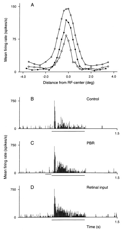
Figure 8. Effect of electrical PBR-stimulation on
the spatial receptive field profile for an on-centre nonlagged Y-cell.
A. Responses to a light slit presented in different position across the
receptive field. The width of the slit was about 1/3 of the width of
the handplotted receptive field centre, the slit length about 3 times
the diameter of the hand-plotted receptive field centre. Each data
point is the average of 5 stimulus presentations. Open circles,
response of the dLGN cell in the control condition, open squares,
retinal input measured by S-potentials. Filled spots, response of dLGN
cell to electrical stimulation of PBR (140 Hz for 70 ms). B-D: Example
of response patterns for the dLGN cell response in the control
condition, with PBR-stimulation, and for the retinal input. The long
horizontal line below the abcissa marks the period when the stimulus
was on, the short bar marks the period with electrical PBR stimulation.
Paul Heggelund (2003)
Signal Processing in the Dorsal Lateral Geniculate Nucleus
Modulation of Neuronal Responses: Implications for Active Vision. (G T
Buracas, O Ruksenas, G M Boyton and T D Albright, eds.) NATO Science
Series 1: Life and Behavioral Sciences 334:109–134.
Page 129
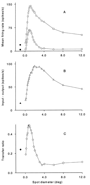
Figure 9. Comparison of the response of an
on-centre X-cell and the response in its retinal input. The stimulus
was a circular light spot of variable diameter but fixed contrast,
centered on the receptive field. A. Open squares, retinal input, open
circles,
dLGN cell response. The response was measured as the average firing
rate during a 500 ms period of spot presentation. Each point is the
average from 20 stimulus presentations. Retinal input was measured as
average frequency of S-potentials. The filled symbols mark spontaneous
activity. B. The difference between retinal input and dLGN cell
response. The data show the reduction in the average response to the
various spot diameters. C. Transfer ratio calculated as output /input
firing rate.
Paul Heggelund (2003)
Signal Processing in the Dorsal Lateral Geniculate Nucleus
Modulation of Neuronal Responses: Implications for Active Vision. (G T
Buracas, O Ruksenas, G M Boyton and T D Albright, eds.) NATO Science
Series 1: Life and Behavioral Sciences 334:109–134.
Page 119
“Neuron model RF-PSTH” and “Neurocluster Brain Model” – are two
different, unrelated models.
The correctness or falseness of “Neuron model RF-PSTH” is completely
unrelated to the correctness or falseness of “Neurocluster Brain Model”.